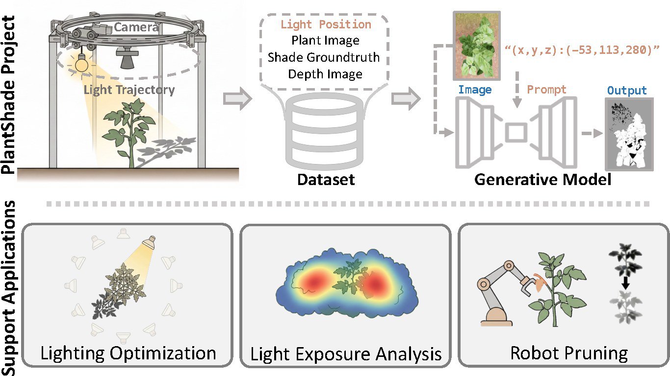
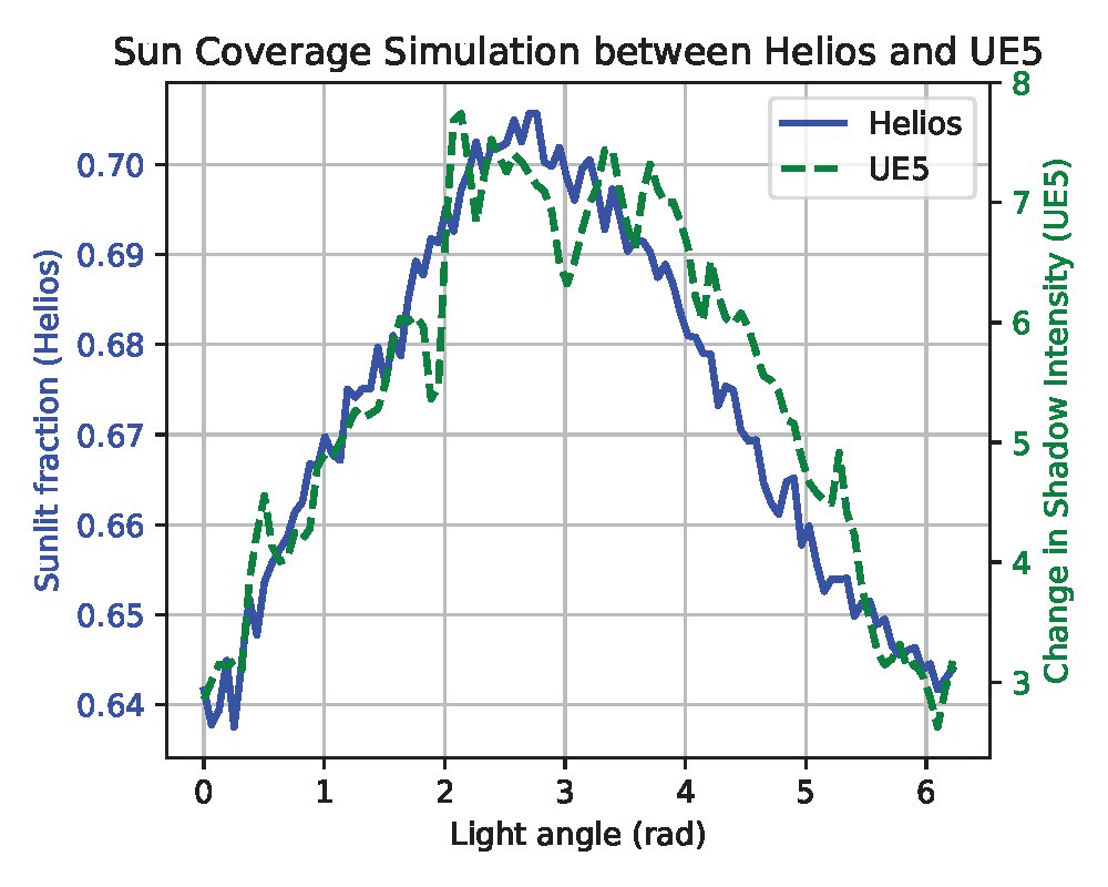
A Helios and UE5 simulation pipeline plus a ControlNet-conditioned diffusion model that generate realistic, time-varying plant shadow maps from a fixed top-down camera, enabling in silico evaluation of supplemental lighting and its downstream effect on canopy photosynthesis.
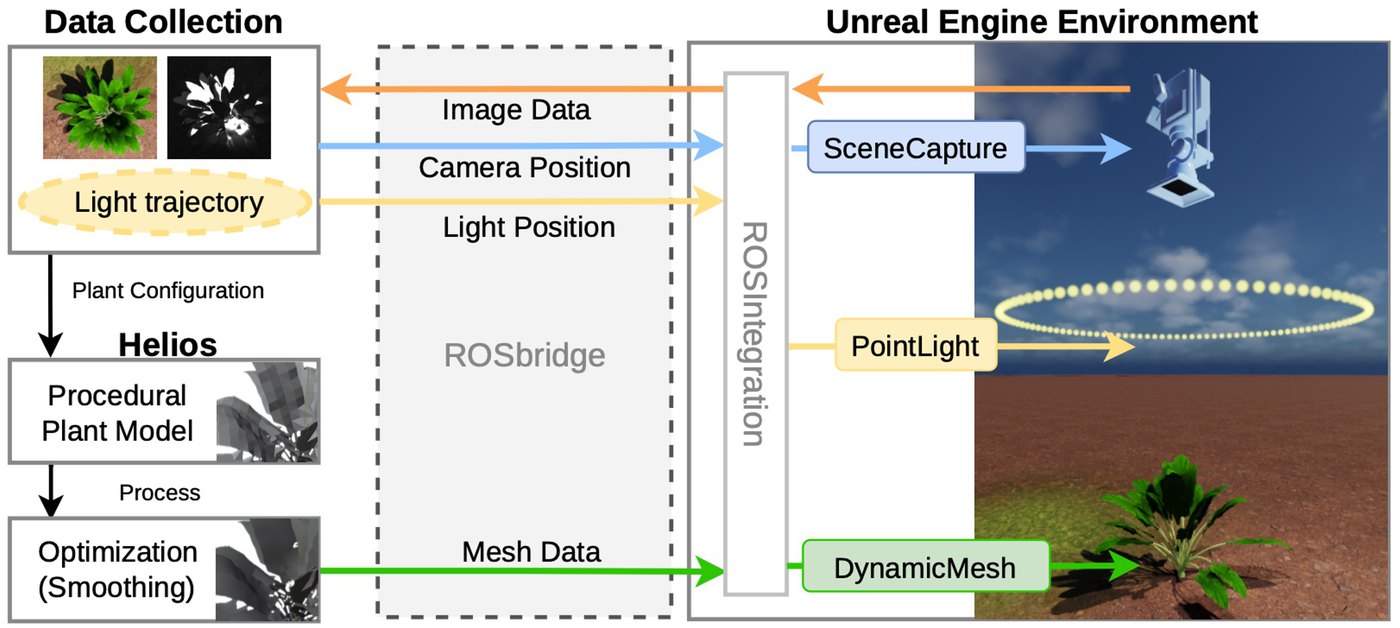
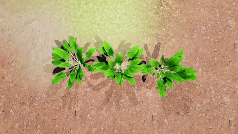
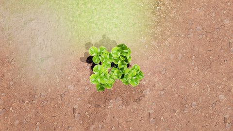
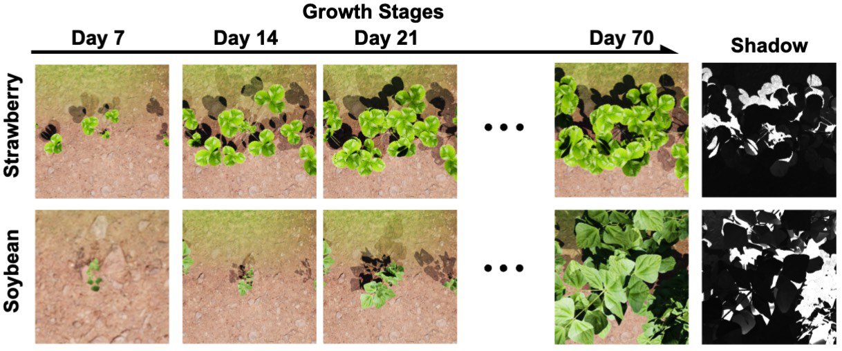
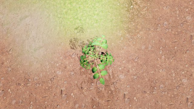
We bridge the biophysical procedural modeling of Helios with the real-time photorealistic rendering of Unreal Engine 5 via ROSbridge/ROSIntegration. Plant meshes (OBJ + MTL) are streamed into UE5 and rendered from a fixed nadir camera, producing aligned RGB, plant-mask, and shadow-intensity ground truth as a supplementary light orbits the canopy.
| Total image pairs | 38,500 |
| Resolution | 1920 × 1080 |
| Camera height | 1.8 m (nadir view) |
| Plant species | Tomato · Soybean · Sugar beet · Strawberry |
| Plant age range | 7 to 119 days |
| Layout configs | 1×1 · 1×3 · 3×5 (50 cm spacing) |
| Solar elevation | 52.24° |
| Supp. light orbit | 1.8 m height · 1.25 m radius · 100 positions |
| Modalities | RGB · Plant mask · Shadow mask · Depth |
After downloading the per-scene zips from the data-collection release, 1_extract_shadow.py turns each
rendered frame into the training target: it thresholds the shadow-intensity render, keeps the plant region,
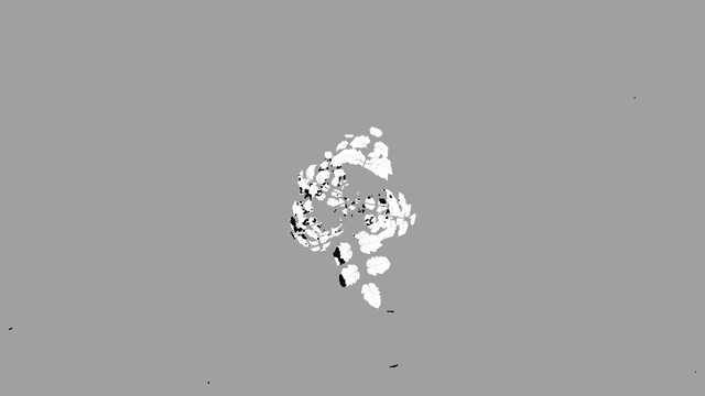
and composites a color-coded map (background #a0a0a0, skeleton #ffffff, shadow
#070707), writing both target/ and the raw targetRaw/. Each sample becomes a
(source, target, prompt) triplet, resized to 512×512, shuffled (seed 42) and split 80/20.
# unzip a scene, then extract shadow maps
unzip data/examples/<scene>.zip -d data/PlantShadeUnzip/

python 1_extract_shadow.py \
    --base_root data/PlantShadeUnzip \
    --out_root  data/shadow
# -> data/shadow/target/ and data/shadow/targetRaw/{"source": ".../seg_54.png", # plant skeleton / edge
"target": ".../target/.../seg_54.png",
"prompt": "122.786 -23.423 280.000"} # light x y z
# pair source/target/prompt, 80/20 split (seed 42)
python 2_build_split.py \
--source_root data/PlantShadeUnzip \
--target_root data/shadow/target --out_dir data30,900 pairs for training and in-domain eval, 7,600 held out for out-of-domain (OOD) evaluation.
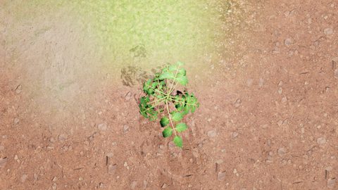
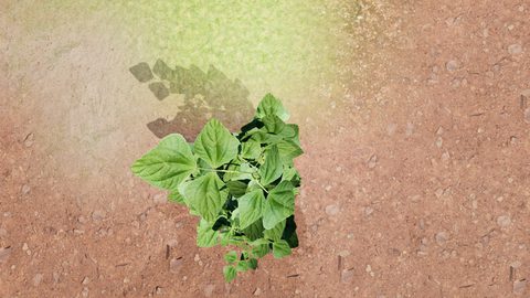
The supplementary light orbits the canopy along a fixed circle (1.25 m radius, 1.8 m height). Pick a layout, then drag the slider or press ▶ Play to move the light through its sampled positions and watch the shadow map evolve for all four crops at a mid growth stage.
A text encoder maps the light-position prompt to an embedding injected via cross-attention, while a ControlNet branch fuses the structural condition (edge/mask) with the appearance prior and guides a Stable Diffusion v2.1 U-Net. Because appearance and structure stay fixed, variation in the output is driven purely by the moving light.
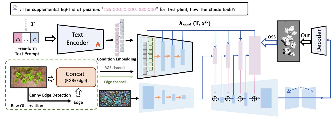
# ControlNet branch on a frozen SD v2.1 backbone
python 3_train.py

# key config (override via env vars)
init_ckpt     = models/control_sd21_ini.ckpt
batch_size    = 16   # PS_BATCH
learning_rate = 1e-5 # PS_LR
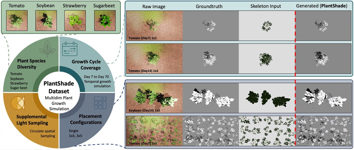
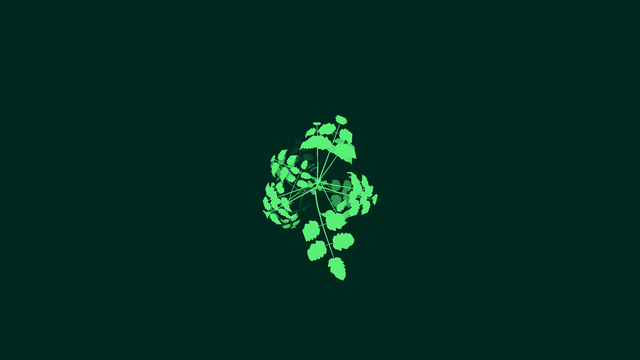
resolution = 512 × 512Given a plant image and a text prompt for the light position, the model generates the shadow map without full 3D rendering. Below are representative cases where the generated shadow closely matches ground truth across the four crops, growth stages, and layouts.
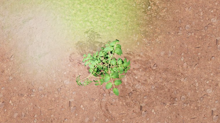
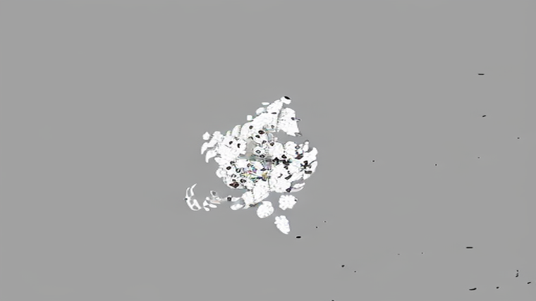
Drag the divider to wipe between the input plant and the model's predicted shadow map. All four are held-out samples generated with DDIM (50 steps, guidance 9.0); predictions are upscaled to the capture resolution.
# checkpoint: huggingface.co/xiao0o0o/PlantShade-ControlNet
PS_CKPT=/path/to/plantshade_epoch51.ckpt \
PS_TEST_JSON=data/test_split.json python 4_infer.py

# key defaults
config      = models/cldm_v21.yaml
ddim_steps  = 50
guidance    = 9.0
shade_thresh = 40
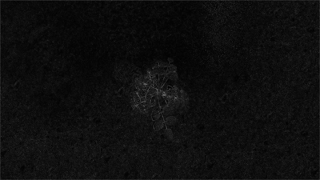
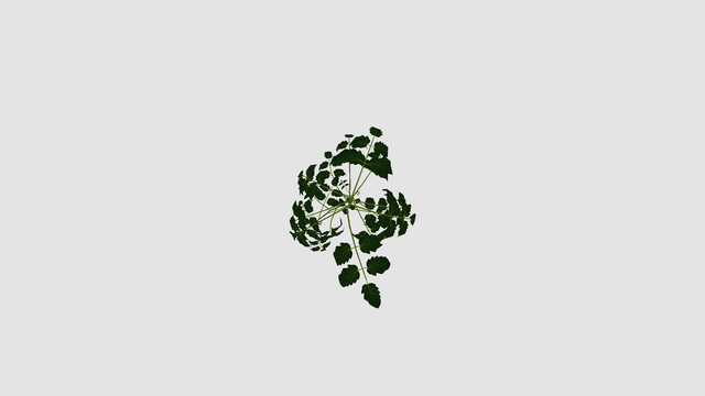
# -> outputs/predictions/generated_*.png (pure) + compare_*.pngEvery capture provides spatially-aligned RGB, structural edges, plant mask, shadow map, and a depth map used downstream for physically-grounded leaf-area and photosynthesis estimation.
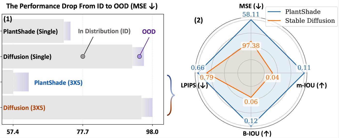
PlantShade vs. a Stable Diffusion baseline across species and layout complexity. Higher is better for mIoU / B-IoU; lower is better for LPIPS / MSE. Columns marked OOD are out-of-domain.
Both methods degrade under OOD placement, confirming the intrinsic difficulty of distribution shift, yet PlantShade keeps a clear margin in every setting.
Predicted shadow maps and rendered depth maps drive a non-rectangular hyperbola (NRH) light-response model. Leaf area comes from depth under a pinhole camera (f=872.72 px); the shaded fraction f weights sunlit vs. shaded photosynthesis into a canopy rate. Explore each species' light-response curve below.
python 5_photosynthesis.py \
    --split data/test_split.json \
    --pred_dir outputs/predictions \
    --output_csv outputs/photosynthesis.csv

def nrh(I, alpha, P_max, theta):        # non-rectangular hyperbola
    a = alpha*I + P_max
    disc = max(a**2 - 4*theta*alpha*I*P_max, 0)
return (a - np.sqrt(disc)) / (2*theta)# leaf area from depth (pinhole, fx=fy=872.72)
A_px = depth**2 / (fx*fy)
A_total = A_px[leaf_mask].sum()
f = A_px[shadow_mask].sum() / A_total # shaded fraction
P_canopy = (1-f)*nrh(I0, ...) + f*nrh(beta*I0, ...)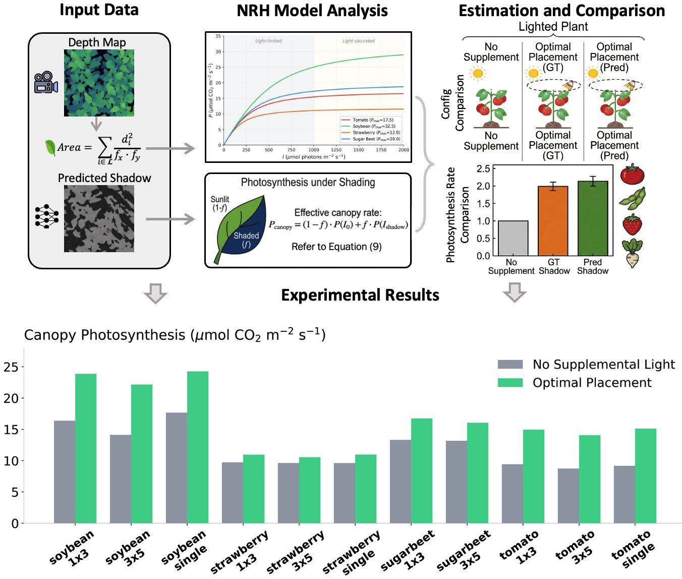
Evaluate light placement and trajectory in silico to maximize canopy photosynthesis before physical deployment.
Spatially-resolved shade sequences inform planting density, row orientation, and sensor placement.
Simulate branch removal to reduce self-shading and improve canopy light uniformity and yield.
Large-scale pixel-aligned RGB/shadow pairs for lighting-invariant robot perception under diverse illumination.
from huggingface_hub import hf_hub_download

# one scene from the dataset
zip_path = hf_hub_download(
    "xiao0o0o/PlantShade",
    "tomato_seed2_14_7_77.zip", repo_type="dataset")

# trained checkpoint (~13 GB)
ckpt = hf_hub_download(
    "xiao0o0o/PlantShade-ControlNet",
"plantshade_epoch51.ckpt")# Helios-UE5 simulator + raw captures
# github.com/ARLabXiang/AgriRoboSimUE5
# releases/tag/plantshade@inproceedings{da2026plantshade,
title = {PlantShade: Predicting Plant Shadows for
Lighting-Aware Robotic Agricultural Operation},
author = {Da, Longchao and Liu, Xiaoou and Li, Xingjian
and Xiang, Lirong and Wei, Hua},
booktitle = {IROS},
year = {2026}
}